The Promises and Pitfalls of Variance Partitioning

Feel free to play around with my code, which is available here.

Some days - between an unchecked global pandemic, the breakdown of voting rights, widespread police brutality, and whatever else is adding stress to your life - the world feels pretty chaotic. But even amid this apparent chaos, our world contains a lot of predictable structure. This is because we’re surrounded by natural covariance: taller people also have bigger feet, fitter people have a lower heart rate, and being outdoors also means being exposed to more light (and Vitamin D!).

Covariance is helpful to us as everyday humans, because it allows us to understand our environment using simple heuristics (buy large socks for tall friends). And covariance is also helpful to us as scientists, because often we can’t directly measure the thing we’re most interested in, like whether someone has been exposed to COVID-19 or how stressed they are. But, we can measure something else that covaries with that thing, like antibodies in the blood or cortisol in the saliva.

All of this natural covariance is useful in that it allows us to understand our surroundings and make scientific progress. But it can also create problems for scientists when we measure several variables that covary and we have to figure out which of these variables is particularly important in explaining our data. To make this concrete, here’s an example: imagine that you want to understand the factors that influence a child’s academic achievement ¹. We know that there is a link between academic achievement and socio-economic status (SES): kids who grow up in wealthier households succeed more in school (Mackey et al., 2015; Rosen et al., 2018). But SES is a very broad term that encompasses lots of factors – which of these factors makes a difference for kids’ performance in school? One reasonable hypothesis is that the amount of time a parent can spend helping their child with homework makes a difference. But maybe the answer really lies in the air quality where they live ². The challenge is that both of these factors are correlated with each other. So, how can we tease them apart - is homework help from a parent or air quality the most important predictor of academic achievement?

Variance partitioning (a.k.a. commonality) analyses are a useful tool that can help us here. These analyses meet the challenge of pulling apart covarying factors by asking: to what extent does each variable explain something unique about academic achievement (that no other measured variables can explain), versus something that is redundant or shared with other variables? Another way of phrasing this is: are homework help and air quality unique or redundant predictors of academic achievement?

But, like most tools, variance partitioning is most informative when it’s applied in the right setting. In this post, I’ll walk you through how to run these analyses in the right settings, and how to avoid using them in the wrong ones. Hopefully, this will make it easier for you to apply this method thoughtfully in your own work.

The Promise and How It Works

The core of variance partitioning rests on regressions. If you’re not already familiar with regressions, they are a way to understand how related certain variables are to the data that you’ve collected. I think the best way to understand regressions is by imagining scatterplots. Say you have some data (observations) and 3 variables (regressors). You can plot the data in a four-dimensional space: 1 axis for the observed value, and 1 for each of the regressors. When you fit a regression, you’re trying to draw a plane through this 4-d cloud of points so that it’s as close as possible to each point in the cloud. If any of the regressors is a good account for the observed data, the resulting regression plane should hew pretty close to the data in that dimension. In other words, such a regressor is explaining a lot of the data’s variance.

Sometimes two regressors account for the data equally well, but it’s unclear whether this is because they’re explaining the same parts of the data (shared variance), or different parts (unique variance). You can also think of this as a venn diagram (Figure 1). Here, the area of the purple circle represents the variance in academic achievement that’s explained by homework help from parents, and the area of the orange circle represents the variance that’s explained by air quality. These circles likely overlap to some extent: the size of the overlapping section represents the amount of variance that’s shared between these variables. However, they probably don’t overlap completely: the portion of each circle outside of that overlap represents the amount of variance that’s unique to that variable.

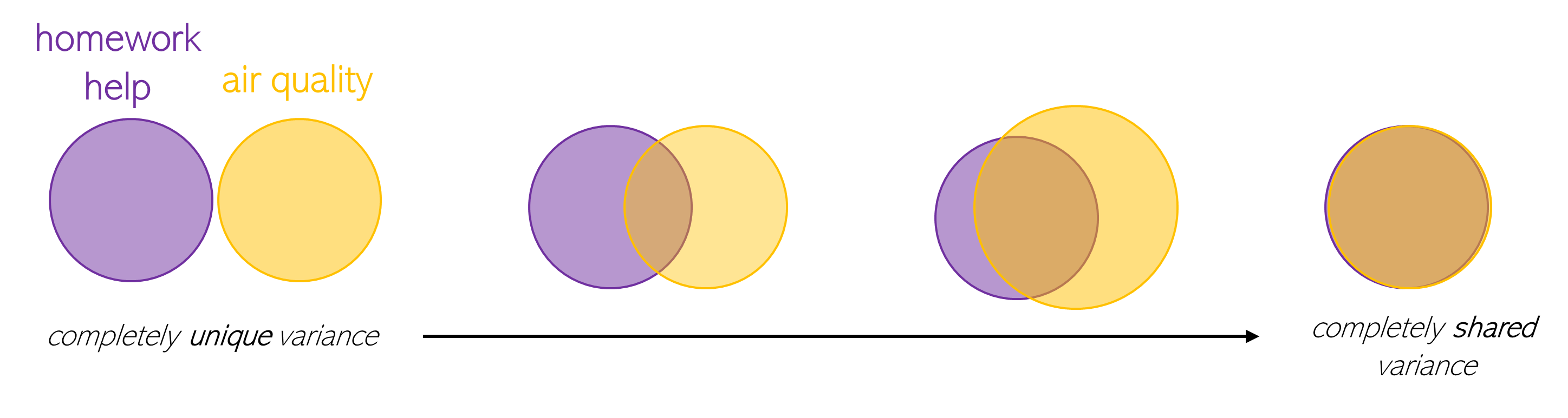
Figure 1. Possible divisions of the shared and unique variance that two variables account for in academic achievement: (1) the amount of homework help a child receives from their parents and (2) the air quality where they live.

Variance partitioning analyses attempt to untangle these two kinds of variance, to understand which variables contribute something unique to the regression’s ability to explain your observed data.

How do you actually calculate shared and unique variance? The first step is to use a series of regressions to predict your data (in this case, academic achievement). These regressions’ regressors are all possible combinations of the variables you’re trying to compare (Figure 2). When comparing two variables (e.g., homework help and air quality), you’ll fit 3 regressions:

1. a regression where the only regressor is homework help
2. a regression where the only regressor is air quality, and
3. a regression where the regressors are homework help and air quality.

For each of these regressions, calculate its r² value, which measures how much of the variance in academic achievement the regression can account for. To get r², fit the regression on a subset of your data (i.e., using k-fold cross-validation, then use the fitted regression to generate predicted values for the data that you held out. Next, correlate those predicted values with the actual, observed data to calculate r. Finally, square that value to get r². The second step is to use the equations in Figure 2 (below) to figure out how much variance is uniquely explained by each variable, and how much is jointly explained by both variables. The result is partitioned variance.

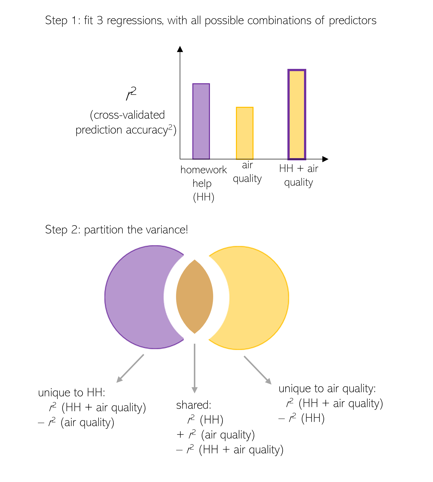
Figure 2. Calculating unique and shared variance (method from Lescroart et al., 2015)

Once you’ve completed these steps, you can interpret the results of a variance partitioning analysis. First, compare how much variance each variable uniquely explained to understand which is the best account for the data. For example, if you found that homework help uniquely explained 30% of the variance in academic achievement, while air quality only explained 5%, that suggests that homework help is a better account for academic achievement than homework help is. It’s also informative to look at the amount of variance that was shared between the variables. For example, if you also found that homework help and air quality jointly explained 20% of the variance, that suggests that air quality is measuring a subset of what homework help is measuring: these variables are highly related, but only homework help is tapping into something extra that helps it explain academic achievement better than air quality. In contrast, if these variables jointly explained 1% of the variance, that would suggest that they are measuring two distinct things, but only homework help can explain academic achievement.

At this point, it’s worth noting that variance partitioning is not the only way to measure how well two variables account for your data – I’ll discuss some alternatives later in this post.

The Pitfalls

While variance partitioning analyses can be a useful way to pull apart the contributions of related variables, it sometimes fails to deliver on its promises. First, it’s not well-suited to comparing more than 3 variables, because the math gets tricky (see Figure 3 for details on how to adapt the method to compare 3 variables). So, if you want to compare the relationships between homework help, air quality, nutrition, and a fourth variable like sleep, I suggest you try a different method (I’ll discuss some examples at the end of this post).

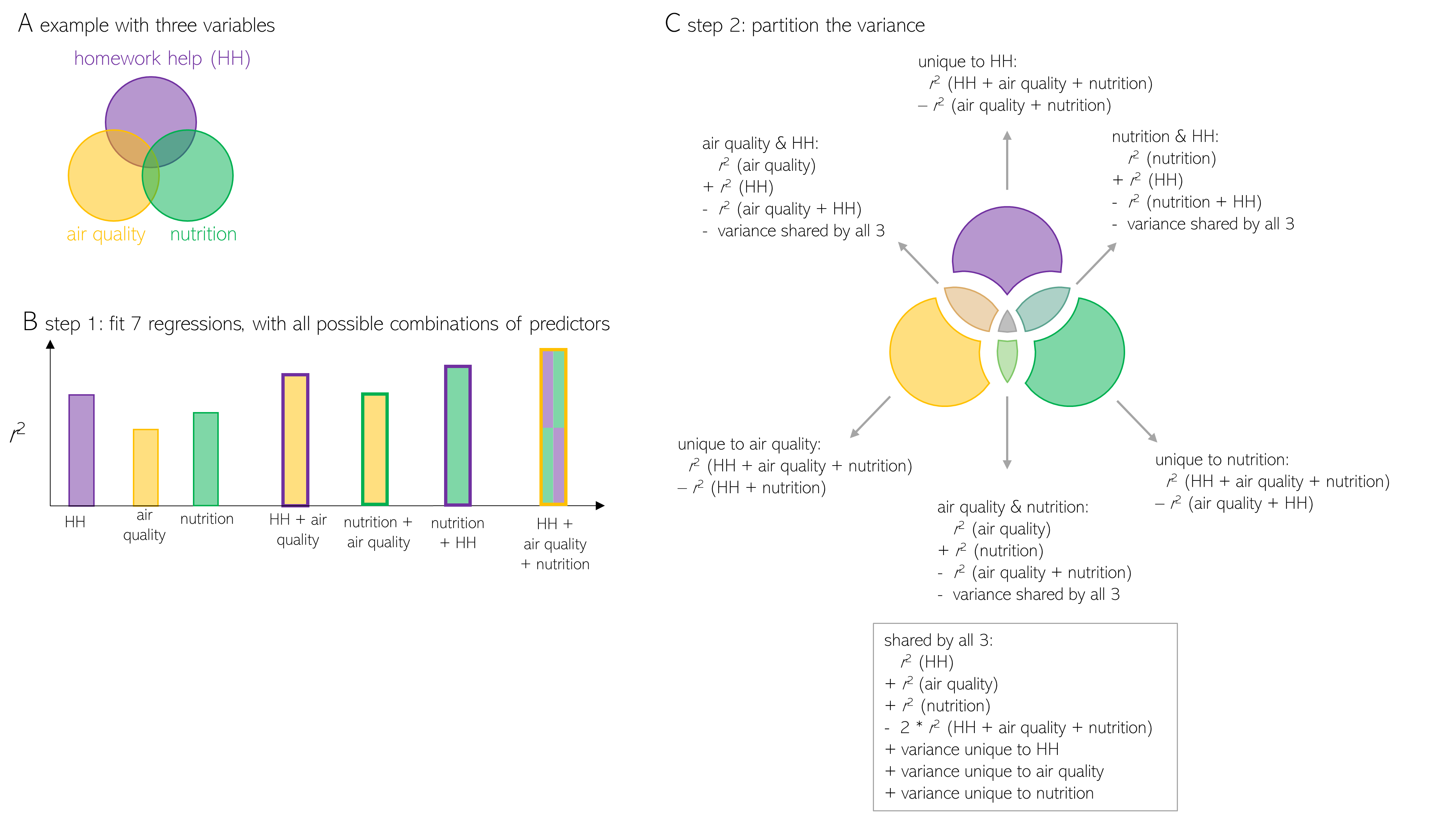
Figure 3. Variance Partitioning analysis comparing 3 variables

Second, sometimes you might find that this analysis yields negative values. Theoretically, this should never happen - a variable can only account for a positive amount of variance in the data. Yet I have found negative variance in my own data, and when I searched for answers I found that this aspect of Variance Partitioning isn’t so well laid-out in the literature. So, what’s actually going on here, and what can you do about it?

In my experience, you can find negative unique or shared variance when the analysis’ subtraction logic breaks down. First, let’s look at negative unique variance. In my own data, I’ve found that this can happen as a result of over-fitting. For example, I ran a neuro-imaging experiment to measure how the brain responded to videos of everyday actions. I wanted to see how well different properties of the videos could predict neural responses to them; specifically, I was interested in the body parts that were involved in the actions, and the body parts that were visible on-screen. As you might imagine, these variables were quite related – in many cases, when a body part was involved in an action it was important enough to be visible in the video – so I used variance partitioning to investigate which brain regions were uniquely explained by one variable or the other. To my surprise, I found that body part involvement uniquely accounted for a negative amount of variance in multiple brain regions.

What caused this negative unique variance? I’m pretty sure that it was the result of using too many redundant regressors, which caused the regressions to over-fit. Variance partitioning analyses assume that there’s no downside to fitting a regression with more variables - a regression based on body part involvement and body part visibility should do at least as well as one based on just body part involvement, if not better. But of course, there are downsides to these extra variables. Specifically, with more variables comes a greater risk of overfitting the data, meaning that the regression has so many degrees of freedom that it can fit a plane to perfectly zig-zag through the data. This hurts the regression’s ability to predict out of sample, resulting in a lower r². Remember that the variance that’s unique to a single variable like homework help is calculated as: r²_{homeworkHelp+airQuality} - r²_airQuality. So, if the regression based on all of the variables is overfit (i.e., has a poor prediction and a low r²), the resulting unique variance will be negative (since r²_airQuality > r²_{homeworkHelp+airQuality}). This is particularly true when a variable is made up of multiple dimensions; in my case, ‘body part involvement’ consisted of involvement ratings for 20 different body parts.

And indeed, I found several signatures of over-fitting in my data. First, my data were vulnerable to over-fitting for two reasons: (1) I was fitting regressions with a lot of regressors relative to the number of observations in the data, and (2) those regressors were correlated with each other (the average variance inflation factor – a measure of the collinearity between regressors – was 129; typically, a VIF > 5 is considered problematic). Both of these things typically cause over-fitting. As a result, the r² for the regression based on both the involved and visible body parts was indeed smaller than the r² values for the regressions based on just one of those variables – which resulted in negative unique variance. Finally, when I ran this analysis using a traditional R² value (the Coefficient of Determination) rather than cross-validated r², the negative variance disappears. Most likely, this happened because R² doesn’t require the regression to predict out of sample, and thus isn’t affected by over-fitting.

At this point, you might be wondering, “can I fix this by using regularized regression?”. This is a natural question because regularized regression is a common tool for avoiding over-fitting. This is because it penalizes the overall size of the weights assigned to each predictor in a regression. To avoid this penalty, a regularized regression will effectively zero out any redundant predictors, which leaves it with fewer degrees of freedom with which to zig-zag perfectly through the data. However, the paper that introduced me to this method discourages using regularized regression to calculate the r² values: “We did not use regularized regression in the current study because the use of regularization complicates interpretation of the variance partitioning analysis” (Lescroart et al., 2015).

So why not take advantage of this tool? Lescroart et al. (2015) don’t expand on their thinking, but I think the answer is that regularized regression introduces more variation across the regressions you fit in the first step of the variance partitioning pipeline. In non-regularized (‘Ordinary Least Squares’) regression, the weights assigned to each regressor may change depending upon which other regressors are used in the regression. That’s because these weights reflect the semi-partial correlations between each regressor and the data being explained – so if you include another regressor that’s very related to this regressor, its weight may shrink. This means that, if you fit 3 different regressions with different combinations of regressors, different weights will be assigned to the regressors in each regression. That is, the weight on air quality might be .8 when it’s the only regressor, and .2 when it’s combined with homework help. Ideally, these weights wouldn’t change too much across regressions, but perhaps some amount of change is inevitable. But, in a regularized regression, these weights can change even more than they would in a non-regularized regression, because the regularization’s weight penalty will affect weights in multi-variable regressions more than in single-variable regressions. As you add more regressors, some weights start to shrink toward zero. That said, I think that it’s worth using regularized regression to avoid getting negative unique variance – which is precisely what happened when I tried this out on my data.

I’ve also found that sometimes negative shared variance can occur. So far, I’ve only observed this in simulations. It seems to specifically occur when comparing two variables that are negatively correlated with each other, or when comparing two highly-correlated variables that are both only moderately correlated with the data you’re explaining. I won’t go into the details here, as I’m not confident that I’ve figured out all the parameters that influence these simulations, but you can check some of them out on my Github repo.

While these pitfalls are problematic, you can avoid them by inspecting your data carefully for tell-tale signals. One signal is finding that the r² value for the regression based on multiple variables is lower than the r² for the regressions based on single variables. In this case, it might be safer to use regularized regressions to calculate the r² values, to avoid negative unique variance. My advice is the same if your regressors are highly collinear (average variance inflation factor > 5). So far, I don’t fully understand the factors that lead to negative shared variance, so I can’t offer solid advice for how to avoid that. Instead, if you find negative shared variance, I think it might be best to turn away from variance partitioning, toward an alternative approach.

Alternative Approaches

There are several alternatives to variance partitioning analyses, which all measure how well two related variables account for the data that you’ve measured. I’ve mentioned a couple of these already. One is semi-partial correlation, which measures the correlation between two variables after removing the effect of a third variable. In fact, this is what a regression does – it calculates a coefficient for each regressor that reflects that regressor’s semi-partial correlation with the observed data. Another is to follow the variance partitioning pipeline, but calculate R² instead of the cross-validated r².

I think that Variance Partitioning based on r² offers at least two benefits over these alternatives. First, this calculation assesses how well each variables can predict your data, which is a more robust test than asking how well they can explain it. If you can predict the data (high r and r² values), you can generalize beyond the data you’ve measured – if you know how polluted a child’s air is, you can say something about how well they’ll do in school. You can’t do this if you’ve merely explained the data (high semi-partial correlation or R²) – you can only say that air quality fits the existing data. Second, the version of Variance Partitioning that I’ve explained in this post makes it easy to compare groups of variables. For example, you could ask how much unique variance a set of variables measuring air quality (e.g., amount of particulate matter, amount of ozone in the air, and the amount of carbon monoxide in the home) accounts for. To do this, just treat each set of variables like a single variable (e.g., run an “air quality” regression with all of these predictors together, instead of a single air quality predictor). This is also true if you’re using R² instead of r² in the variance partitioning pipeline, but it’s not true if you’re using semi-partial correlations.

Two other alternative analyses are a Bayesian method (Diedrichsen & Kriegeskorte, 2017) and ZCA-whitening (e.g., Green & Hansen, 2020). I haven’t looked deeply into either of these methods yet, but they seem promising.

Finally, it’s sometimes possible to design an experiment so that you can directly compare variables without specialized analyses. For example, imagine that you’re designing a neuroscience experiment to ask what brain regions respond to pictures of toys. But, most toys are colorful and you want to be sure that you’re not unintentionally studying responses to color. To solve this, you could use greyscale photos of toys in your experiment. Or, you could design an intervention study – for example, install air filters in the homes of 100 children and observe whether their academic performance improves, even if the amount of homework help they get doesn’t change. Unfortunately, careful experimental design is not a panacea. It’s quite challenge to control every covarying variable, and doing so may result in non-naturalistic data (if people are used to looking at colorful toys, their brains may respond differently to grey-scale ones).

Conclusions

You’ve now stuck with me through a pretty long post – so here’s one last piece of advice. When interpreting variance partitioning results, pay attention to which variables accounted for the most unique variance, but don’t put too much stock in the overall amount of variance they explain. I found that when you change details in the analysis – using cross-validated r² or R², regularized or un-regularized regression – the exact amounts of unique and shared variance also change. For example, homework help might uniquely account for 20% of the variance in academic achievement in one analysis, but 15% in another. In general, it seems like the overall patterns remain stable – homework help accounts for more unique variance than air quality, regardless of the analysis. So when comparing analyses across papers or datasets, pay attention to which variables accounted for the most unique variance but not how much unique variance they accounted for.

Taking all of this together, I think that variance partitioning analyses can be a useful tool – when used thoughtfully. The ‘thoughtful use’ part is key, and it’s the reason this blog post ended up being much longer than I expected! But I hope that the strategies I outlined above for inspecting your data will be helpful for that endeavour.