In my last blog post, I described how Wasserstein (a.k.a. Earth-Mover’s) distances could be used to measure the dissimilarity between two neural response patterns. The main benefit of “Brain-Mover’s Distance” is that it takes the topology of the brain into account, measuring not just how similarly the voxels in question respond, but also their proximity in the brain. I also worked through an example to demonstrate how this method could be used to assess the replicability or inter-subject reliability of an fMRI dataset.
In this post, I’ll work through a second example, demonstrating another natural application for this distance metric: Representational Similarity Analyses (RSA). RSA is a method for understanding the representational geometry of a brain region - for example, whether it distinguishes between two categories or sub-divides them into four. The general method is as follows:
Calculate a neural representational dissimilarity matrix (RDM) for a region of the brain. This RDM is a square matrix, with one row for every item in your fMRI experiment. For example, if you showed participants images of 50 animals and 50 objects, your RDM’s dimensions would be 100 x 100*. Each cell (i, j) in the RDM stores the dissimilarity between that region’s responses to item i and item j - for example, between a picture of a football and a picture of a kitten.
As I covered in my previous blog post, dissimilarity could be measured in many ways (1-correlation, squared Euclidean distance, Mahalanobis distance, etc.). Regardless of the dissimilarity metric, the RDM is said to reflect the region’s representational rules. So, if the region represents animals and objects differently, then the RDM should show that all animals are similar to each other, and all objects are similar to each other, but animals and objects are not similar.
Calculate a comparison RDM, measuring the similarity between the same items on some other basis. The best comparison will depend upon your question. If you’re curious whether this brain region houses the mental representations that inform behavior, consider calculating the comparison from behavioral data, such as reaction times in a visual search experiment or physical distances in an intuitive arrangement task (Cohen et al., 2016; Mur et al., 2012). If you’re more interested in characterizing the kinds of information that are represented in this region, it might be better to use some hypothesized features, such as the items’ animacy or size. In general, this comparison RDM should be something that you understand better than the brain, so that your results are interpretable.
Compare the neural RDM and the comparison RDM. This is typically done by correlating the two matrices (using only one triangle of the matrices and excluding the main diagonals). If the correlation is high, that suggests that the neural representational geometry resembles the comparison’s representational geometry.
*Note that if your fMRI experiment used a blocked design, these dimensions might be much smaller. For this reason, it is crucial to do RSA only on data with a relatively high number of conditions - my rule of thumb is at least 8.
So, what happens if you use Brain-Mover’s Distance to calculate the neural RDM, versus a more standard metric like correlation distance? I’m inclined to believe that Brain-Mover’s Distance might capture the true neural similarity structure better than other common metrics, because it takes the brain’s topography into account. Of course, it’s difficult to test this prediction because we don’t actually know what the true structure is! Instead, the first step is to test whether RSA results will differ depending upon whether correlation distance or brain-mover’s distance is used to calculate the neural RDM.
The Data
To explore the effect that Brain-Mover’s Distance has on RSA, I analyzed some fMRI and behavioral data from my former lab-mate Caterina Magri and my advisor Talia Konkle. The fMRI data were collected while subjects viewed 72 everyday objects, like a clock and a grill. I examined responses to these objects in voxels in the ventral occipito-temporal cortex that responded reliably over the course of the experiment (Tarhan & Konkle, 2019).
The behavioral data were collected from a visual search experiment. On each trial, subjects saw a circular array of 6 images (1 target image and 5 identical distractors) and were asked to detect the odd image out. The resulting reaction times indicate the visual similarity of the target and distractor images - a longer reaction time indicates more similar-looking images. These reaction times were log-transformed and then submitted to a mixed-effect model to partial out single-subject variability, ultimately producing a group-level behavioral RDM. There was no overlap between the subjects who completed the fMRI and visual search experiments.
The Analysis
Next, I conducted two versions of RSA. In one, I calculated each subject’s neural RDM using Brain-Mover’s Distance. Then, I correlated each of those neural RDMs with the behavioral comparison RDM (Figure 1a). The second version followed the same process, except that I calculated the neural RDMs using correlation distance. My code for all of this is up on Github here.
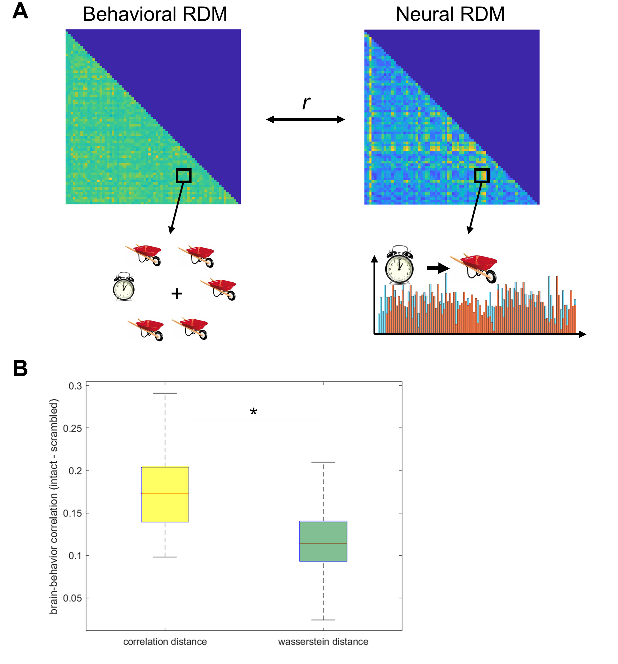 Figure 1. Wasserstein Distance as a measure of neural dissimilarity. (a) Representational Similarity Analysis compared the neural dissimilarity matrices in each subject’s ventral OTC with a behavioral dissimilarity matrix based on visual search data. (b) The brain-behavior correlations were significantly lower when neural dissimilarity was measured with wasserstein distance than correlation distance. Asterisk indicates significant paired-sampled t-test (p < 0.001).
Figure 1b shows the brain-behavior correlations using the two methods. Interestingly, these dissimilarity metrics do make a difference: brain-behavior correlations were significantly lower when the neural RDM was calculated using Brain-Mover’s Distance than correlation distance (t(9) = 6.67, p < 0.001).
What does that mean?
This is an intriguing result, but what does it mean? Did Brain-Mover’s Distance capture the true neural dissimilarities better than correlation distance, and reveal that they are less similar to behavior than we might have thought? Or did correlation distance get closer to the truth? Since we still don’t know the ground truth, at this point all we can really say is that they differed. To understand what might cause these two metrics to produce different results, we’ll need to do some digging.
Some possible shovels
One way to dig is to adopt a simulation-based approach. This would allow you to specify several versions of ground-truth, and then ask: what kinds of neural responses lead to different RSA results?
To start, what’s the effect of how the multi-voxel response pattern is distributed within the region you’re investigating? Will correlation and Brain-Mover’s Distance measure different similarity structures if the response pattern is like a gaussian (high response in the middle of the region, dropping off as you move away from the peak voxel)? What about a salt-and-pepper pattern? To dig into these questions, I would start by specifying three response shapes: a single gaussian, stripes, and salt-and-pepper (Figure 2a). For each of those shapes, randomly generate 100 slightly-different response patterns. The idea is that all of these variations within a shape should seem intuitively similar to each other - all of the gaussian patterns should look similar, but the gaussians shouldn’t look similar to the stripes. Then, calculate the correlation and brain-mover’s distances among the patterns for each shape. If you normalize the distances so that correlations and wassersteins are on the same scale, are the patterns more similar when measured with one metric than the other (Figure 2b)? Does the answer change depending upon the shape? Next, to assess whether these metrics do equally well at distinguishing the three hypothesized shapes from one another, make a 3x3 RDM. Cells on the main diagonal will contain the same information as in Figure 2b. The off-diagonal cells will compare two different shapes - how similar are stripes and gaussians? Ideally, the off-diagonal distances will be much higher than the on-diagonal distances. But it will be informative to see whether the two distance metrics will both produce that pattern.
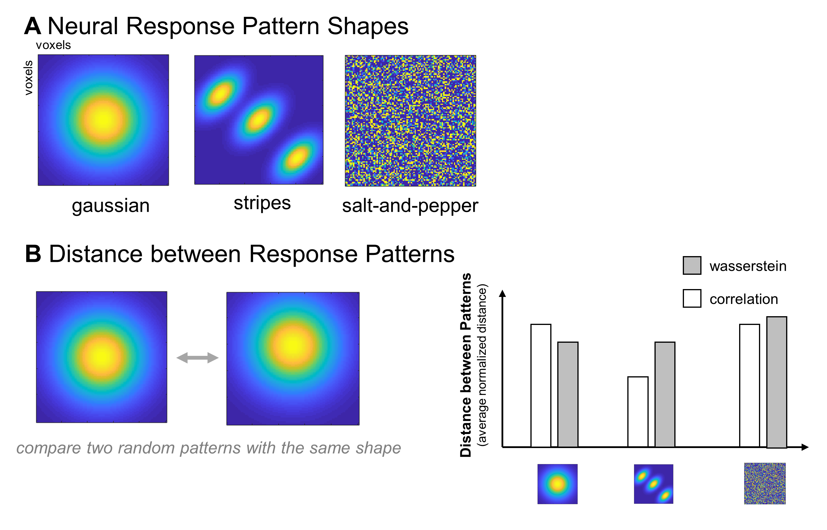 Figure 2. Ideas for how to use simulations to characterize situations in which correlation distance and Wasserstein distance differ. (a) Examples of three possible response pattern “shapes”: gaussians, stripes, and salt-and-pepper. An example pattern is shown for each shape, in a simulated square region of interest. Brighter colors indicate simulated voxels that responded highly to this item, while cooler colors indicate voxels that did not respond much to this item. (b) Sketch of an analysis to determine whether correlation and Wasserstein distance diverge more for some response pattern shapes than others: random jitters of the same shape are compared using both metrics, over many iterations.
In addition to their shape, what’s the effect of shifting response patterns slightly within the brain region? In theory, such a shift should affect the correlation distance more than the Brain-Mover’s Distance. You could test this by smoothly varying the amount of offset between two patterns of a given shape and calculating the distance between the patterns at every step. This would produce a smooth curve for each distance metric (Figure 3), which would give you a clearer idea of how changes in a pattern’s location affect the neural RDM under each metric.
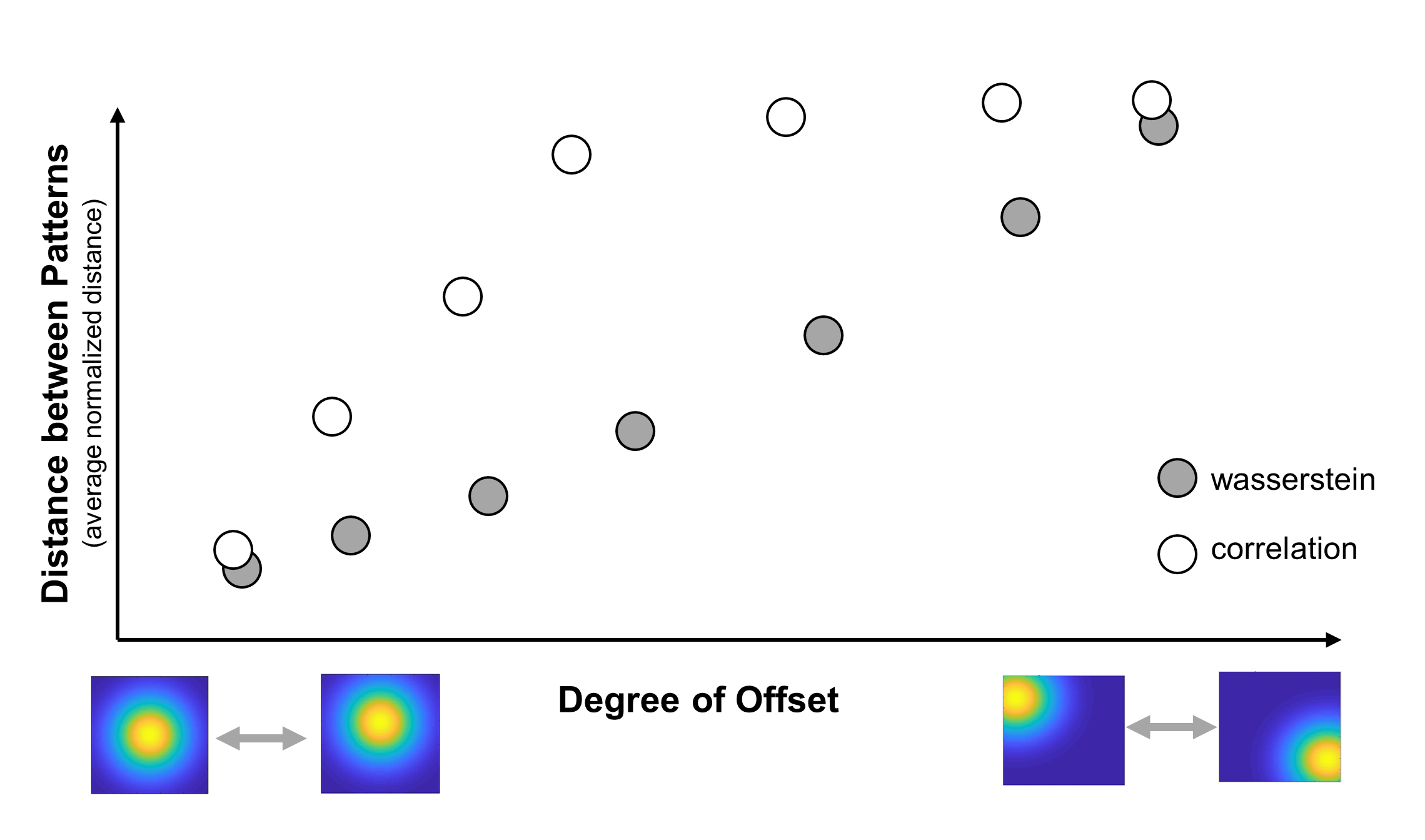 Figure 3. Example analysis to characterize how the degree of spatial offset between two response patterns affects Wasserstein and correlation distances between those patterns.
Taken together, these simulations are meant to elucidate the conditions under which correlation distance and Brain-Mover’s Distance differ, and which metric better captures researchers’ intuitive notions of neural similarity. Of course, it’s important to think deeply about what “neural similarity” means to you before embarking on this analysis - are two patterns similar if they are close together in the brain? If they’re offset by one millimeter, are they still reasonably similar? What about 5? Does their distribution within the region matter at all? What about their extent? I suspect that researchers vary a lot in their answers to these questions.
Going Further
Once we understand the conditions under which these distance metrics produce different estimates of neural similarity, the question of which is a more accurate estimate of the true relationship between the brain and behavior still looms. This could be addressed with still more simulations - somehow specify a series of “true” behavioral and neural RDMs, then test which distance metric gets you closest to that truth. Of course, these simulations alone will not be conclusive. To come to a generalizable conclusion about what Brain-Mover’s Distance captures in RSA, you would also need to examine other brain regions, other behavioral tasks, and other datasets. In addition, it’s important to compare Brain-Mover’s Distance to other distance metrics, beyond correlation - for example, cross-validated Mahalanobis distance has been getting a lot of good press lately (e.g., Walther et al., 2016). I think this is a fascinating field, and there’s still so much work to do that it’s a little dizzying. So, while I don’t expect to follow this line any further, if you take a stab and find something, let me know! I’d love to live vicariously through you.