When analyzing fMRI data, we often seek to measure similarity between two brain responses. For example, we run reliability analyses to ask, “how similar is this subject’s brain when they see the same image again?” or “how similar is this subject to the rest of the group?” Relatedly, Representational Similarity Analyses (RSA) allow us to ask, “Does this brain region respond the same way to all members of a category - like inanimate objects?” All of these questions are based on the same understanding of “similarity:” the extent to which the same voxels respond a lot, a little, or not at all in two samples of the data. This notion of similarity is ubiquitous in fMRI analyses; therefore, it’s extremely valuable to find the best way to measure it.
In pursuit of this goal, researchers have adopted several different similarity metrics. The current toolbox includes correlation (of which there are many variants: Pearson, Spearman, Kendall’s tau-a.), Euclidean distance, and Mahalanobis distance. But how can we tell which of these are useful – what makes a similarity metric “good?” I think that four considerations determine the goodness of a similarity metric:
The metric should capture the similarity between patterns of responses (e.g., among multiple voxels) not just in main effects. Correlations, Mahalanobis distance, and Euclidean distance all check this box, but Euclidean distance is influenced by both similarity in patterns and main effects.
The outcome should be interpretable within the context of the data. I think some of the methods in the toolbox accomplish this better than others; for example, correlation is easy to interpret because it has a restricted range and (somewhat-) agreed-upon standards for what constitutes a “big” or “small” effect. However, Euclidean distance is less intuitive because it’s unclear how to map a unit of distance onto the physical space of the brain.
A similarity metric should be computationally tractable. By this I mean that it should be possible to calculate it on a standard laptop, and it shouldn’t take more than a couple of days at most.
Most controversially, I argue that a distance metric should take the geometry of the brain into account.
Why Does Geometry Matter?
Much research has established that the brain has a meaningful topographic organization: for example, Early Visual Cortex is organized into alternating zones of preference for vertical and horizontal orientations, and these zones are separated by sharp borders (DeYoe et al., 1996). Similarly, high-level visual cortex can be subdivided into alternating zones that prefer big objects, small objects, and animals (Konkle & Oliva, 2012; Konkle & Caramazza, 2013). Therefore, it is important to consider how spatially close or distant response patterns are in the brain, in addition to the similarity of their response patterns. None of the methods in the current toolbox take this geometry into account: if two response patterns are offset by 5 voxels or 50, they are considered equally distant.
Wasserstein Distance
However, there is another similarity metric that does take geometry into account: Wasserstein Distance. Wasserstein distance (a.k.a. “Earth-Mover’s Distance”) calculates the cost of moving one distribution of data to another, taking spatial proximity into account (Figure 1). When applied to the brain, this method asks: how far (in millimeters) would you need to move one unit of activation to transform one response pattern into another? It’s as if one activation pattern is several piles of dirt, the other pattern is several holes, and you have to move the dirt into the holes. This metric thus meets all four criteria outlined above: it measures similarity between response patterns in an interpretable unit, is computationally tractable, and takes the brain’s geometry into account. This metric has not been broadly used in cognitive neuroscience, partly because it is computationally intensive in large datasets. However, with a few mathematical tricks (and with the help of this toolbox that I’ve implemented in MATLAB), this metric can be applied to a number of fMRI analysis settings.
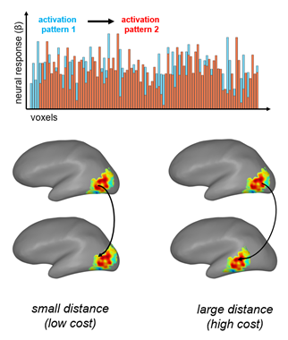 Figure 1. Wasserstein Distance calculates the difference between two multi-voxel activation patterns as the cost to transform one pattern of responses across voxels (shown here in blue) into the other pattern (orange). Thus, if the activation pattern is shifted by a small amount within the brain, the distance will be low. If it is shifted by a large amount, it will be high
How Does it Work?
First, a primer on the shape of fMRI data: in general, we measure responses in the whole brain to a set of stimuli. The brain is divided up into a large number of voxels (3-dimensional pixels, measuring roughly 1-3mm in each dimension), so our data live in a matrix whose dimensions are # of stimuli by # of voxels. A response pattern is a vector of responses to a single stimulus in some set of these voxels (for example, all the voxels in early visual cortex).
To calculate a Wasserstein Distance between response patterns in the brain, you need two things:
A matrix of multi-voxel activation patterns in response to a set of stimuli
A matrix of actual distances (in millimeters) between all the voxels in your data. In my toolbox, I measured these as Euclidean, straight-line distances (so two voxels on opposite sides of a sulcus would be very close). You could also use cortical distance (those same voxels would be further apart) or even distances along white-matter tracts! The point is that these distances reflect actual locations in the brain.
With these two pieces of data in hand, the next step is to solve an optimization problem - the heart of the Wasserstein calculation. In this problem, we’re asking how costly it would be to transform one activation pattern into the other, so that in the end the first activation pattern looks exactly like the second - the same amount of activation in the same voxels. To imagine this a little more concretely, recall the dirt-and-holes analogy I described before, where one activation pattern is the piles of dirt and the other is the holes. Two things determine the distance between the dirt and the holes: how close the holes and the dirt are to each other, and how well the size of the holes matches the size of the dirt. If the holes are near the dirt (the two activation patterns are spatially similar), you don’t have to do much work - the earth-mover’s distance is low. If the holes are far from the dirt (the activation patterns are spatially dissimilar), the distance is greater. In addition, the relative sizes of the dirt and the holes matter: if each pile is close to an equally-sized hole, the distance is low. But if some piles are larger than their nearby holes, you’ll fill up the closest holes and then have to carry some dirt further to fill additional holes - the distance is greater. To put that back into brain terms, if the two multi-voxel patterns have roughly the same amount of activation in nearby voxels, the distance is low; however, if they have different amounts of activation, the distance is high.
Of course, there are many ways to transform one pattern into another, some more efficient than others. So in calculating the Wasserstein Distance between the patterns, we’re searching for the transformation that requires the minimum work - the shortest distance needed to move all of the dirt into the holes. That will be the “Brain-Mover’s Distance” between our patterns. A nice feature of this method is that the units are interpretable: Brain-Mover’s Distance is measured as the minimum distance (in millimeters) that we’d have to move one unit of activation (such as a beta weight) to match the two activation patterns.
A Quick Caveat It’s worth pointing out here that there’s an ambiguity to Wasserstein Distances: a given distance could reflect spatial dissimilarity, pattern dissimilarity, or some combination of the two. Goodman (1972) criticized the ways we talk about similarity for exactly this reason - we say that two things are “similar,” but we don’t specify on what basis they’re similar. Most similarity metrics suffer from this ambiguity; for example, a correlation coefficient doesn’t tell you which voxels responded in the same way across the two patterns. The question here is not whether similarity is a useful concept, but what definition of similarity is most useful in the context of fMRI analysis. Thus, it’s worth considering whether Wasserstein Distance tells us something interesting about patterns in the brain that existing metrics do not. Nonetheless, it will also be useful to explore the different interpretations of a Wasserstein Distance (whether it reflects spatial dissimilarity, pattern dissimilarity, or a combination) and consider whether these can be grouped into a single notion of similarity.
How Can You Use It?
So, how and when can you use “Brain-Mover’s Distance?” Here are some ideas:
Assess the replicability of your data: how consistent are neural response across subjects?
Compare two groups: How similarly do blind and sighted brains respond to object names?
Compare large-scale preference maps across conditions: how similar are the zones of cortex that prefer big or small objects when you show people full photographs vs. unrecognizable metamers (e.g., Long et al., 2018)?
Representational Similarity Analysis: does a brain region respond one way to all animals, and a different way to all objects?
Region-of-Interest (ROI) locations: is the Fusiform Face Area in the same location in children and adults?
As you can see, there are many potential applications for this tool. I’ll start by demonstrating one use-case: assessing the replicability of my data. In a subsequent blog post, I’ll explore a second: Representational Similarity Analysis. Both of these are well-documented in my toolbox, but I’ll explore their interpretation in greater depth here.
Use Case 1: Replicability
The Question
I set out on this analysis because of a nagging doubt about my data. I had run 13 subjects on an fMRI experiment, in which they watched short videos of 120 everyday actions (Tarhan & Konkle, 2019). That’s not a lot of subjects. This small N was especially worrisome because we keep seeing new evidence that fMRI data aren’t very replicable, even in much larger samples (e.g., Eklund et al., 2016; Turner et al., 2018). Had I collected enough data to trust any of my results?
To answer this troubling question, I asked: how consistent were neural responses across subjects? If their responses all followed the same pattern across my conditions - e.g., their motion-sensitive areas all responded most to videos with a lot of movement but face-sensitive areas responded most to videos with prominent faces - then I would consider my data to be reasonable replicable. You could also think of this as “inter-subject reliability,” but here I’ll use “replicability” because I refer to a different sense of reliability later in this post. If my data were replicable, then I could be reasonably confident that my analyses of the group data were based on something real, rather than being driven by flukes and outliers. If, however, I observed a lot of variance in the group, I would need to collect more data.
The Nitty-Gritty
There are a few ways to test this, but I settled on a split-half analysis: over many iterations, I split my 13 subjects into 2 groups (of 6 or 7 subjects) and calculated an average response matrix for each group. Then I computed the Wasserstein Distance between the two groups for each condition (in this case, an action video).
The full analysis took about 24 hours to run on a standard computer, without any parallelization. This datum links all the way back to the beginning of this post: a similarity metric should be computationally tractable. Brain-Mover’s Distance is computationally tractable, but only with a few crucial tricks:
Select a sub-set of the brain. At the resolution of my data (3mm isotropic voxels), the brain contains about 100,000 voxels. I ran this analysis in a small subset of that: roughly 8,000 reliable voxels that I previously identified. You can find more details about how I identified those voxels here and in Tarhan & Konkle (2019, BioRXiv); the key is that these voxels responded consistently within subjects, and I conducted all of my analyses in these same voxels.
Meta-voxelize the data. Even with my reliable subset, it would have taken about a week to analyze 8,000 voxels. So, I down-sampled my data into “meta-voxels,” which each contained 8 original voxels (2 x 2 x 2).
Specify a sparse network. Realistically, there’s no reason to calculate the distance between two voxels at opposite ends of the brain. Instead, you can specify a sparsely-connected network: each node of the network is a voxel, each edge connects two voxels together, and activation can only be moved between voxels that are connected. Figure 2 illustrates the sparse network used in this analysis: the result has a lot of local connections between spatially-close voxels but fewer long-range connections between far-apart voxels. This step is optional, but it does speed things up because the optimization problem considers fewer potential solutions, making the computation about 3 seconds faster per condition (which added up to about 10 hours across all of my conditions and iterations). It’s also important to note that you might calculate slightly different distances using a fully-connected network. But if so, using a sparse network will result in a slight over-estimate, resulting in a more pessimistic evaluation of the data’s replicability.
Findings
So, were my data replicable or did I need to run more subjects? The results are plotted in green in Figure 2: the average Brain-Mover’s distance between halves of the data was around 3.6 mm, meaning that matching one half of the data to the other would require moving each unit of brain activation at least 3.6 mm through the brain.
How do we know if this is a high or low distance? Unlike correlation distance, Wasserstein Distance doesn’t have a strict upper bound, so it’s harder to apply standards for what constitutes a “big” or “small” effect. So, to establish a baseline, I ran the same analysis on scrambled data (which should not be replicable). Those results are plotted in gray (Figure 2). As you can see, the Brain-Mover’s distance is noticeably higher when the data are scrambled (t(119) = 41.02, p < 0.001). This is a huge effect, which I also validated in a separate analysis using correlation distance (t(119) = 229.4, p < 0.001). On the strength of these results, I now feel pretty good about the replicability of my data.
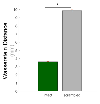 Figure 2. Results of the analysis using Wasserstein distance to measure the replicability of the raw fMRI data in a sample dataset. Asterisk denotes a significant paired-sampled t-test (p < 0.001).
Interpretation
Given previously-published findings (e.g., Turner et al., 2018), it’s somewhat surprising that my data were so replicable. What explains this difference? One possibility is that it’s the distance metric - maybe assessing replicability using correlation distances (as Turner et al. did) unfairly deflates the estimate of replicability, because small shifts in activation patterns across subjects are treated as totally different data. But this is an unlikely explanation, because I found similar results using correlation distance. Instead, I think the key difference between my analysis and Turner et al.’s is the brain region. I restricted my analyses to a subset of voxels that responded reliably within subjects, across odd and even runs of the experiment. This was a natural choice for me to assess the replicability of my experimental results, because I restricted all of my analyses to these voxels. In contrast, Turner et al.’s main analyses were based on the whole brain.
This is a meaningful difference that highlights the importance of thoughtfully choosing which regions of the brain to analyze. There are many possible ways to go about this, depending in part upon the researcher’s question. For example, if the question is about exactly how a known region responds to different kinds of stimuli, it makes sense to define a Region of Interest. In contrast, if the aim is to characterize large-scale maps in the visual cortex, it makes more sense to select voxels based on their reliability, activity, or variance (e.g., Kriegeskorte et al., 2008; Pereira et al., 2009; Tarhan & Konkle, 2019). Researchers who don’t select a specific region to analyze, and instead conduct a whole-brain analysis, run the risk of including noisier regions whose responses are not very replicable, and thus may find that their results are less robust (as Turner et al. did). Another factor shown to affect replicability is the amount of data collected per subject (Nee, 2019). These data may have been more robust because they were collected from about 25 minutes of scanning, compared to 10 minutes in Turner et al.
It might seem circular to assess replicability using reliable voxels - aren’t reliable voxels selected to be replicable? Not exactly. Reliable voxels are selected within each subject, so they reflect the regions that respond consistently across time, not across subjects. Indeed, I’ve observed a fair amount of variability between subjects in the location and extent of their reliable voxels. In this case, I defined reliable voxels using the group data (otherwise, it would be very difficult to compare activation patterns across subjects). However, this selection method still doesn’t guarantee that the data will be consistent across subjects. Given that replicability may be better among carefully-selected regions than in the whole brain, we should take Turner et al.’s results with a grain of salt. Many researchers do choose their brain regions carefully, and therefore their results may be much more replicable than these pessimistic findings suggest.
Finally, how important is it that I chose reliable voxels? How would these results change if I chose a different meaningful set of voxels, such as those that are more active during the experiment than at rest (Kriegeskorte et al., 2008; Konkle & Oliva, 2012; Mur et al., 2013; Jozwick et al., 2016; Kay et al., 2017)? This is an open question, but I suspect that the replicability would still be high within active voxels because activity (based on a t-value) does take noise into account. However, it’s definitely worth investigating this empirically.
Is it okay to compare voxels in different regions?
Some might object to this analysis, because it’s a common principle in cognitive neuroscience that you shouldn’t compare responses across different regions of the brain, which may have different signal strengths. We know that the amount of signal measured using fMRI can vary drastically over the brain (Eklund et al., 2016). As a result, some regions have a higher average response across stimuli than other regions. Therefore, comparing the average response to a condition, such as scenes, in two different regions is ill-advised: a difference might exist simply because of differences in their baseline response strengths.
Does the same danger exist when comparing two multi-voxel response patterns, which stretch over far-apart regions of the brain? I don’t believe that it does, because this amounts to a comparison between the same set of voxels. Imagine that these voxels include some in the parietal lobe and some in the ventral visual cortex. The signal is much stronger in the parietal lobe, because it’s closer to the receiver coil that encases the subject’s head during the experiment. So, when I compare all of these voxels’ responses within the two subject groups, the parietal voxels will always have more activation than the ventral visual ones - the piles of dirt are higher there. That might mean that more activation is moved from parietal voxels to another location than is moved from ventral voxels. But these voxels should have more dirt in both groups - so differences in overall activation across regions shouldn’t affect your estimate of the replicability. Finally, in this case it’s helpful to remember that this same concern should apply to an analysis using correlation, rather than Wasserstein distance - if you’re comfortable using correlations to calculate the replicability of your data, then you should feel similarly about Wasserstein distance.
Conclusions
To conclude, Brain-Mover’s Distance applies a well-studied mathematical method to calculate the similarity between neural responses. Its emphasis on topography makes it well-suited to a wide range of fMRI analyses - here, I’ve described one in depth, but there are so many more possible applications! In my next post, I’ll tackle another use case: Representational Similarity Analysis (RSA). This will be a more complicated story, and I’m curious to see if others can shed light on some of its more puzzling twists.