When researchers measure neural responses using fMRI, they’re often faced with a question: which brain regions should they analyze? There’s no single best answer to this question, but I recently published a paper (with my advisor, Talia Konkle) outlining one approach: selecting the voxels with reliable data. The aim is to restrict your analyses to the parts of the brain that respond consistently over multiple presentations of the same stimuli. Essentially, we do this by calculating each voxel’s split-half reliability (how similar the voxel’s profile of responses to all the stimuli is in two halves of the data). Then, we use a data-driven method to select a reasonable cutoff for which voxels are reliable enough to include in the final analysis.
Since publishing this paper, several people have approached me with questions about how to adapt this method to their particular constraints, many of which I had never considered! So, I’ve gathered some of the most interesting and relevant questions here as a sort of epilogue to the paper. Feel free to email me if you have additional questions that aren’t answered here or in the paper!
1. Do you have code to implement this method?
Yes! Check out the Open Science Framework for code and the data from the paper.
2. Should I define one set of reliable voxels for the group, or do it separately for each subject?
This is a great question whose answer really depends upon the final analysis. If you intend to analyze group-level data, then it makes sense to also use group-level data to define a single set of reliable voxels. However, if you plan to run single-subject analyses, then it makes more sense to define reliable voxels separately in each subject.
One important note here is that if you define reliable voxels separately in each subject, you might end up with coverage in different regions for different subjects. We’ve found that the extent and location of reliable voxels varies a lot across individuals; for example, here are the reliability maps from two different subjects who completed the same experiment (Tarhan & Konkle, 2019, BioRXiv):
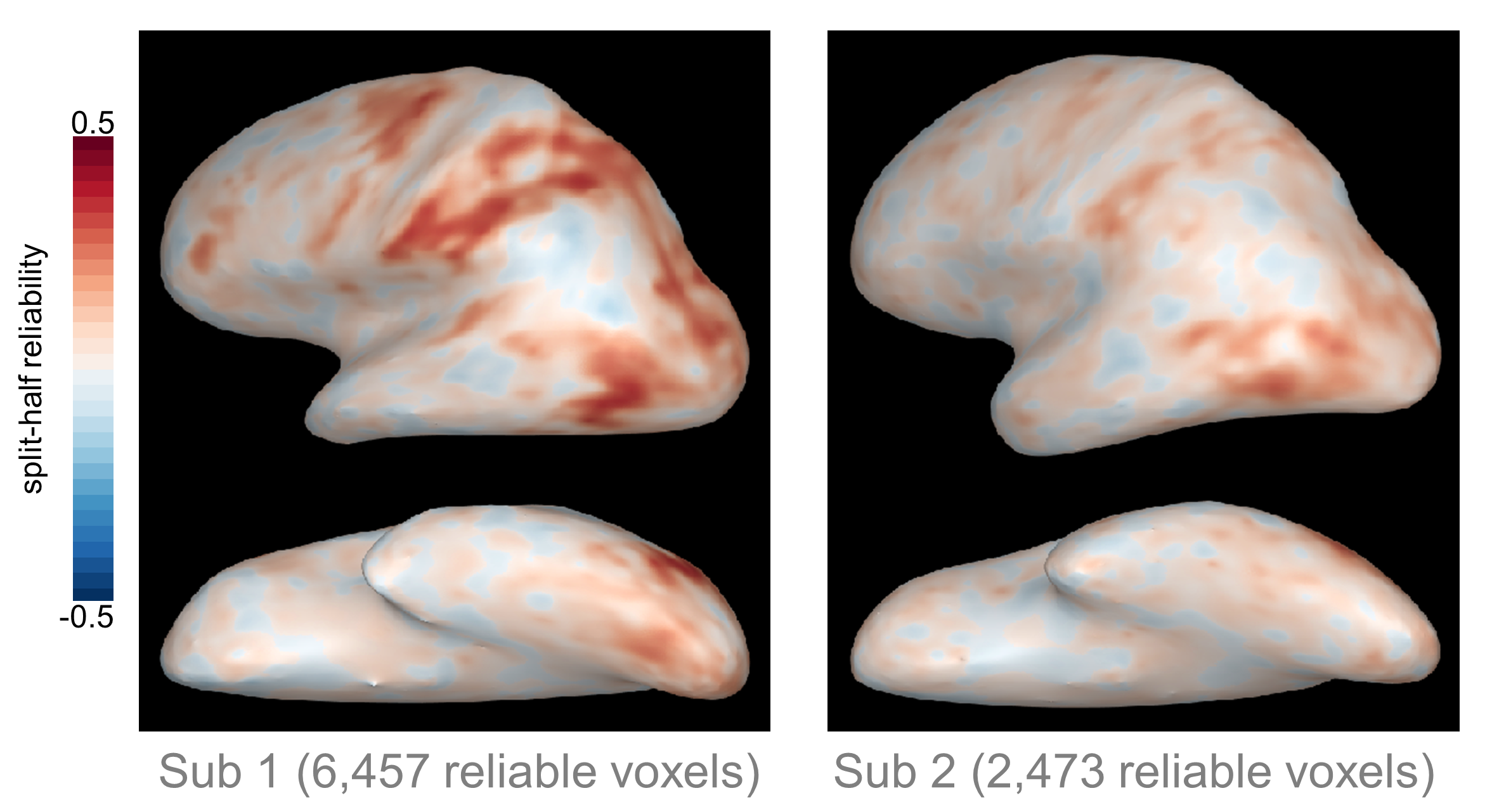 As you can see, in Subject 1 roughly three times as many voxels survived the reliability-based cutoff compared to Subject 2. It’s not just that Subject 2 had fewer voxels in the same regions as Subject 1. Instead, whole regions - such as the intraparietal sulcus and ventral occipito-temporal cortex - were missing from Subject 2’s reliable coverage, but present for Subject 1.
This variation means that you have to be thoughtful when interpreting single-subject results. If you define reliable voxels separately in each subject, you may not be able to compare results in the same regions across all subjects. One alternative is to define a single set of reliable voxels using group-level data, then analyze each subject’s data within those voxels. In this case, it’s easier to compare the same regions across subjects; however, it’s important to keep in mind that in some cases you may be analyzing unreliable data. For this reason, it’s useful to include a figure with each subject’s reliability map for reference when presenting the data.
3. How many conditions do I need in my design to use this method?
The short answer is that you need at least 15 conditions.
The long answer is that the reliability analysis rests on a correlation measure: each voxel’s split-half reliability is calculated by correlating its responses in odd and even scanning runs. Correlations are rather unstable with small datasets - changing one or two datapoints can significantly change the correlation coefficient.
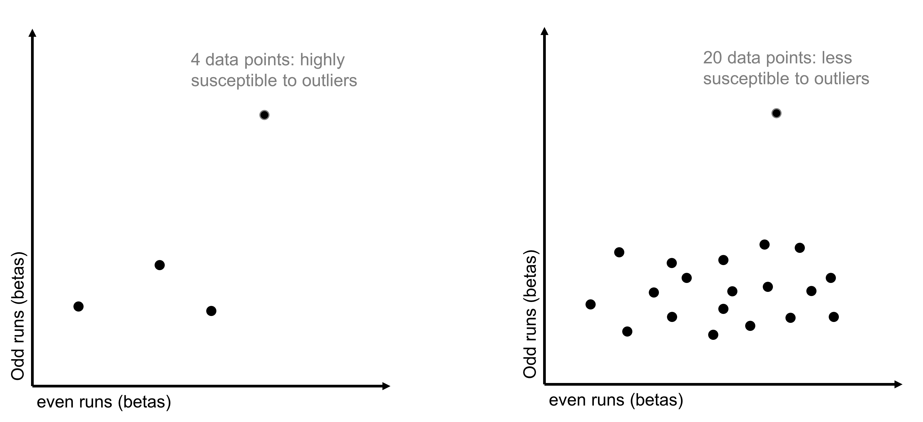
Figure 2: Correlation Stability
Therefore, the key question here is, how many conditions do you need to calculate a stable correlation? To estimate the answer, we ran some simulations over an example dataset with 60 conditions. For every possible number of conditions from 1 to 60, we randomly drew a subset of data of that size 100 times. For each iteration, we calculated the split-half reliability of that subset of data and then got the standard deviation of the distribution of correlations that was built up over the 100 iterations. As expected, the standard deviation was higher - split-half reliability was noisier - when we sampled fewer conditions. But we found that it stabilized around 15 conditions, and this finding replicated in a separate dataset. You can find more details about this analysis in our paper (linked above).
Of course, 15 is the minimum - more is better!
4. I don’t have 15 conditions - what do I do?
If you’re using a blocked design with fewer than 15 conditions, consider whether you could convert it to a “mini-blocked” design instead. For example, say you have blocks of objects, faces, and scenes and the blocks are 20 seconds each. You could break up each block into 4 5-second “mini-blocks” that contain multiple presentations of the same stimulus (or category of stimulus). For example, in one “object” mini-block you could flash an image of scissors on and off 5 times. Or, you could present 5 different images of scissors. You could do the same for mugs in another mini-block. If you enter the mini-blocks as regressors in a GLM to estimate the voxels’ responses, you’ll get a separate estimate (e.g., a beta) for each mini-block.
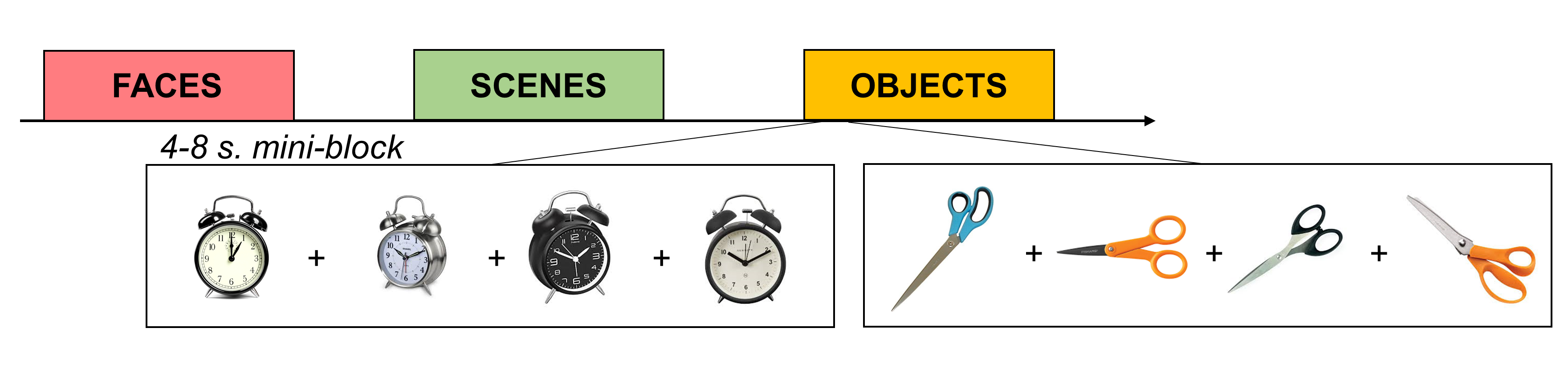
Figure 3: Mini-Blocked Designs
Note that this isn’t quite the same as an event-related design, which typically contains much faster blocks (e.g., 1-2 seconds). In our data, we’ve found that using intermediate-length mini-blocks boosts our signal-to-noise ratio far above what we could measure with a fast event-related paradigm (a topic for another blog post).
5. Can I concatenate the data from all runs for a single subject to get more conditions?
When we calculate split-half reliability, we first estimate each voxel’s responses during all odd-numbered scanning runs and all even-numbered runs. We do this by computing a GLM over the data from all of the relevant runs and including “run” as a separate regressor. You could achieve a similar result by calculating neural responses separately for each run and then averaging across runs. To make this more concrete, say I have data from 8 scanning runs, with the same 20 conditions per run. After aggregating over all odd and all even runs, I get 20 data points for each half of the data, which I’ll correlate to estimate split-half reliability.
Rather than aggregating over runs, some people have asked whether they can increase the amount of data that they enter into the split-half correlation by concatenating together the data from all odd runs and all even runs. So, in the same example experiment, you could concatenate together the data from all four odd runs and get 80 data points, then do the same for the even runs. 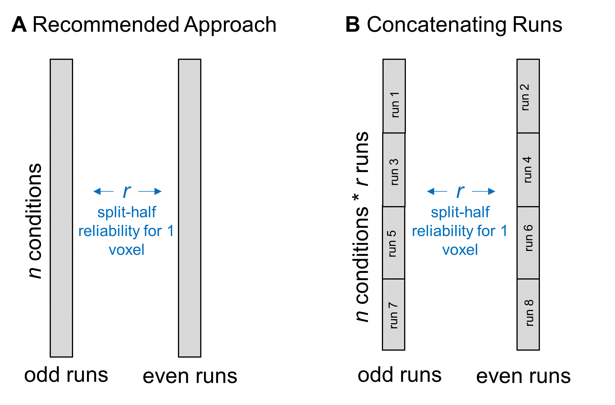 I don’t recommend this strategy for two reasons. First, aggregating over runs increases your power. Any small variations in response magnitude will get washed away in the average, which should make your more confident in the reliability results. Second, one of the assumptions of a correlation is that each observation is independent. If you include multiple measurements of the same condition in this calculation, it may bias the result to be stronger than it truly is.
6. Can I concatenate the data from all of my subjects to get more conditions?
In a similar vein, some people have asked whether they could increase the data entered into the split-half correlation by concatenating together all subjects’ responses. For example, if I have 6 conditions in my experiment and 10 subjects, I could correlate all subjects’ responses in even runs (60 data points) with their responses in odd runs (also 60 data points).
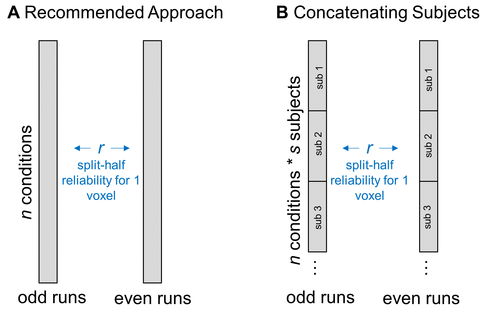
Figure 5: Concatenating Data across Subjects
This is an interesting approach, and may be a reasonable way to go if your aim is to analyze a single, constrained region that you know is responding reliably in all of your subjects. However, if your aim is to map out the functional properties of a large swathe of cortex, this approach might limit your coverage too much. That’s because, as I mentioned above, subjects can vary a lot in how reliable a given voxel is. If some regions have reliable coverage in some but not all subjects, this method might constrict your coverage so that it doesn’t cover any of those regions, resulting in a highly focal set of regions rather than a large swathe of cortex. But, there’s another reason I hesitate about using this method: I can think of a couple of situations in which correlating responses that have been concatenated over subjects might either over- or under-estimate a voxel’s reliability. In the first case, imagine a voxel that is highly reliable in each subject, so that the scatterplot between odd- and even-run betas (where each dot is a condition) is basically a straight line for each subject. But now imagine that, although all subjects are perfectly reliable, their average activation across conditions is different – so, when you make a scatterplot of responses to all conditions, from all subjects, you’d get something like Figure 6a:
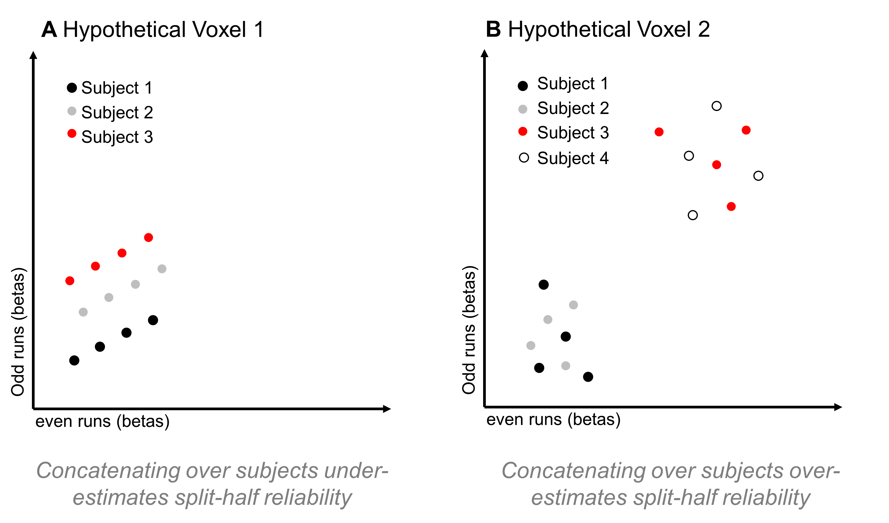
Figure 6: Hypothetical Problems for Concatenating across Subjects
In this case, computing the correlation over that point cloud might result in a rather low r-value, leading you to conclude that the voxel isn’t reliable, even though if you looked at the responses within each subject (and had enough conditions to compute a stable correlation), you’d find that it is reliable.
In the second case, imagine a voxel that actually isn’t reliable at all – if you looked at single-subject data, you would find a low correlation between odd- and even-run responses in every subject (Figure 6b). But, on top of that, imagine again that some subjects have a fairly high average response across conditions, while others have a fairly low average response across conditions. That might result in a scatterplot with two clusters – the high-response subjects form a cluster in the upper right of the plot, while the low-response subjects form a cluster in the lower left of the plot. If you computed a correlation over all of that data, I would expect that it would be high; however, if you computed a correlation on a by-subject basis, it would be low.
Of course, these are just hypotheticals, and I haven’t worked through whether they are likely in fMRI data. However, they seem plausible enough to give me pause about using this method. I think a better approach is to increase the number of conditions in your data by implementing a mini-blocked design (see above).
7. Can I use this for a searchlight analysis?
Absolutely! Although our paper focuses on the case of calculating the reliability of a voxel’s response profile, it’s also possible to calculate the reliability of the searchlight RDM centered on that voxel (or, “search-sphere reliability”). This approach can also buy you more conditions, in a sense. Instead of correlating odd- and even-run responses to n conditions, you’re correlating odd- and even-run similarities between (n choose 2) pairs. Calculating reliability based on single voxels or search spheres will probably yield a similar set of voxels, but the results will be slightly smoothed when using the search sphere approach. You can see this effect in the example below, where I calculated reliability for the same subject using both methods:
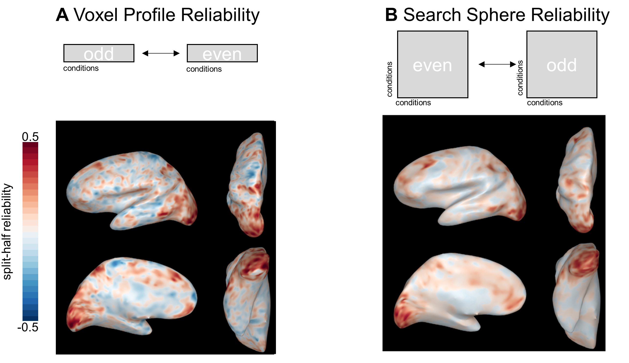
Figure 7: Voxel-Profile and Search Sphere Reliability
8. Do I need separate data to define the voxels and run my analyses?
This turned out to be a surprisingly complicated question, and we’re grateful to a very thoughtful reviewer for shedding light on its complexity. After exploring our data in a few ways, we think that it’s safe to use the same data to define reliable voxels and analyze their data if you’re performing single-voxel analyses (e.g., voxel-wise encoding modeling). However, if you’re running an analysis over a collection of voxels (e.g., representational similarity analysis or decoding), doing so can bias your results. So, if you plan to run multi-voxel analyses like RSA or decoding, we suggest that you use one of two approaches to separate the processes of defining the voxels and analyzing their data. The most conservative approach is to use totally separate data for each step. An alternative, which preserves more power, is to use a jackknife approach: for example, in a pairwise decoding analysis, define the reliable voxels using all data except for the pair of conditions being decoded. Then, decode those conditions in the held-out data, using that set of voxels.